Efficiency of Road Networks

April, 2021

For any two points on the Earth, the geodesic (as the crow flies) distance between them is usually different from the travel distance (along roads). For example, the fastest driving route from Boston to Dallas is about 1750 miles long, but the geodesic distance between Boston and Dallas (as the crow flies) is only about 1520 miles. Ignoring practicality, there could have been a perfectly straight road directly from Boston to Dallas, in which case the travel distance would equal the straight line or geodesic distance. In that sense, real-world road networks are not perfectly efficient because drivers have to take routes which are not perfectly straight lines from origin to destination.

The efficiency of a route can be measured by computing the geodesic distance divided by the route length. In the case above, because the route from Boston to Dallas is about 1750 miles long and the geodesic between Boston and Dallas is about 1520 miles, the route efficiency is \(1520/1750 = 0.869\). If a route were perfectly direct, then its efficiency (by this measure) would be 1. If it were twice as long as a perfectly direct route, then its efficiency would be 0.5. In general, if a route is x times as long as the geodesic between its endpoints, then its efficiency is \(1/x\).

There is an important distinction between the shortest route and the fastest route. For this project, I used the fastest route because that is what real drivers use. However, the same methods can be used for shortest routes.

Route efficiency is useful for a number of reasons. Here are a few examples:

• It is often simpler to compute the geodesic distance than it is to compute the travel distance, so the geodesic distance is often used as an approximation of the route distance. By looking at the distribution of route efficiencies for millions of routes, we can check whether the geodesic distance is a good approximation of the travel distance.
• Route length is closely related to fuel consumption, which is in turn related to cost, and so route efficiency is important for logistics.
• By looking at how route efficiency varies with geodesic distance, it is possible to study some of the scale-free properties of road networks.

Computing Route Efficiency on a Large Scale

In order to measure the efficiency of an entire road network, as opposed to the efficiency of a single route, I compute the route efficiencies for a large number of random routes within the area of interest. More specifically, I generate thousands to millions of pairs of population-weighted random points within the target area, compute the fastest routes between those pairs of points, compute the route efficiencies of those routes, and take the mean. It is important that the random points be generated proportional to population because otherwise some sparely populated territories (i.e. northern Canada or Siberia) have a disproportionate impact on the analysis. Conveniently, this measure can also be interpreted as the expected value of route efficiency between any two randomly chosen people within the area of interest.

The first step in computing the route efficiency of a road network is to generate population-weighted pairs of points. By “population-weighted”, I mean that the probability of picking a point in some region is proportional to the population of that region, so that the distribution of points roughly matches the distribution of people (see the figure below for an example in the United States). I used the highest-resolution gridded population estimates from SEDAC, which aggregates data from censuses around the world. This would probably be unnecessary if the goal were only to look at travel efficiency within a single country, but having population data from a consistent source for the whole Earth is important for looking at route efficiency in places like Europe where the road network crosses national borders. The figure below shows 2000 population-weighted random points in the contiguous United States:

The next step in computing route efficiency of a road network is routing. For this, I used OSRM with data from OpenStreetMap (OSM). I decided to focus on North America and Europe because these are the places where OSM has the best coverage. That said, the OSM files for these regions are altogether about 35GB, and OSRM’s preprocessing phase requires a huge amount of RAM on these large files, so I had to do the preprocessing on EC2.

Before routing, each randomly selected point is snapped to the nearest point on the road network. If the nearest point on the road network is more than 5km away from the original point, then it is removed from the results.

Results

I started by computing the route efficiency between 4 million population-weighted pairs of points in the contiguous United States. Below is a histogram of the results:

The mean route efficiency is 0.843 with a standard deviation of 0.045. This means that if you chose two (uniformly) random people in the United States, and asked one to drive to the other, the distance between them would be about 84% of the route length. Because the standard deviation is so low, this estimate is surprisingly accurate.

Next, I computed a similar set of route efficiencies for pairs of points in Europe. The histogram below compares the distribution of route efficiencies in the United States with that in Europe:

The results are surprisingly different, with the mean route efficiency in Europe being only 0.767. My first hypothesis for the discrepancy was that many geodesics in Europe go over water, and so (without extensive bridges) travel distance is often forced to be longer than the geodesic distance. Consider, for example, the geodesic and fastest route from Rome to Athens:

More formally, land in Europe is more concave than the United States, and so geodesics (which can cross water) are generally straighter than travel routes (which generally cannot cross water). In the example above, a route from Rome to Athens cannot be direct because it would have to go through the sea, but similar situations are rare in the roughly convex United States.

However, that hypothesis became less convincing when I compared individual European countries (which are more convex than Europe as a whole) with US states, and saw that some of the disparity remains:

Above, we see that some states (like Massachusetts) show similar results to European countries, but that others (like Illinois and California) still show a disparity. It seems here that route efficiency roughly correlated with population density, or maybe with the age of the road networks (older resulting in lower route efficiency).

Route efficiency vs distance

Next, I looked at how route efficiency varies with geodesic distance. The plot below shows route efficiency as a function of geodesic distance in the US and Europe:

The results are mostly flat, especially in the US, meaning short routes are about as efficient as long ones, which aligns with some theories about the scale-free properties of road networks. There is a noticeable dip in efficiency for the longest routes, but this is probably an artifact of the small number of routes which are so long, together with the fact that the extreme longest routes generally have endpoints on peninsulas or in other unusual geographic situations. There is also a dip for the shortest routes, which can be seen better with this zoomed-in version of the above plot:

Here we can see that there is another regime governing routes within 5 miles or so, where short routes are less efficient than longer ones. Zooming-in further, we see that there is yet another regime governing even shorter routes within a radius of 0.2 miles or so:

So to summarize, there seem to be three regimes of route efficiencies. For routes longer than about 5 miles, route efficiency is largely independent of route length. For routes between 0.2 and 5 miles, longer routes are more efficient, but with diminishing returns. For routes shorter than 0.2 miles, shorter routes are more efficient.

In order to understand how these regimes come about, I generated visualizations of some example routes at these different scales:

With these maps, it was possible to come up with some hypotheses about the different regimes. The short-scale routes are small enough to consist of a single road segment with few turns, in which case it is unsurprising that the resulting routes are straight. These routes are smaller than the feature size of the road network, and so they are trivially efficient.

Mid-scale routes involve intracity travel. They are long enough that there is no single road from origin to destination, but short enough that there are only a handful of route choices. For these, it is worth it to take large roads, but there may only be a single viable choice, leading to inefficient routes. Otherwise, they are left navigating smaller roads which are often laid out in patterns (e.g. grids) that also lead to inefficient routes.

Long-scale routes involve intercity travel, and are long enough to have a selection of large roads to follow, allowing for more direct routes.

Time efficiency

Next, I looked at a variant of route efficiency which is based on travel time instead of distance. Instead of computing the geodesic length divided by the route length, I computed the geodesic length divided by the route duration. This measure of time efficiency is just the distance traveled divided by the time, so it can also be interpreted as the magnitude of the mean velocity in the direction of the destination. For example, Boston and Chicago are about 856 miles apart, and the fastest route from Boston to Chicago takes about 16.5 hours, so the time efficiency is 856/16.5 mph = 51.9 mph, which is the magnitude of the mean velocity on that fastest route.

Time efficiency and route efficiency each have their own uses. Route efficiency measures the directness of a route, and it approximates the excess resources (like fuel) needed to move on the travel network compared with geodesics. Time efficiency, on the other hand, measures how fast a driver can move on the road network. For some uses, travel distance is more important (like a logistics company trying to minimize fuel consumption), and for others travel time is more important (like a commuter trying to minimize their time on the road). Much of the analysis for route efficiency can also be done with time efficiency, so here I reproduce some of the most important route efficiency results with time efficiency.

Below are histograms showing the distributions of time efficiency for the United States and Europe. The results are similar to route efficiency, except Europe’s mean is slightly closer to the US’s:

As with route efficiency, these distributions are relatively tight, with almost all routes in the US having a time efficiency between 40 and 50 mph.

The plots below show time efficiency as a function of geodesic distance, zoomed-in to the scales at which the three different regimes operated for route efficiency:

The long, mid, and short regimes still appear just like with route efficiency, although their behavior is slightly different. In the long-range regime, time efficiency takes longer to level off, with a significant slope even at 500 miles. This means that longer routes generally have higher time efficiency, which is expected because longer routes spend more time on the biggest and fastest roads. In contrast, route efficiency levels off faster because there are some scale-free properties of the layout of roads, but speeds are not scale-free.

In the short-range regime, the peak around 0 is lower magnitude, which makes sense because even though small roads might be straight, they have low speed limits.

Local route efficiency

Finally, I looked at how route efficiency varies with geography. Up to this point, I had only looked at the mean route efficiency on the scale of countries or states, but I wanted to see how route efficiency varies on smaller scales, and how it interacts with geographic phenomena like mountains, cities, or country borders.

In order to compute the local route efficiency at a point \(p\), I generated a disk centered on \(p\) with radius 50 miles, computed 10000 routes between population-weighted points in that disk, and took the mean. I did this for 10000 uniformly placed points in the contiguous United States, and plotted the results:

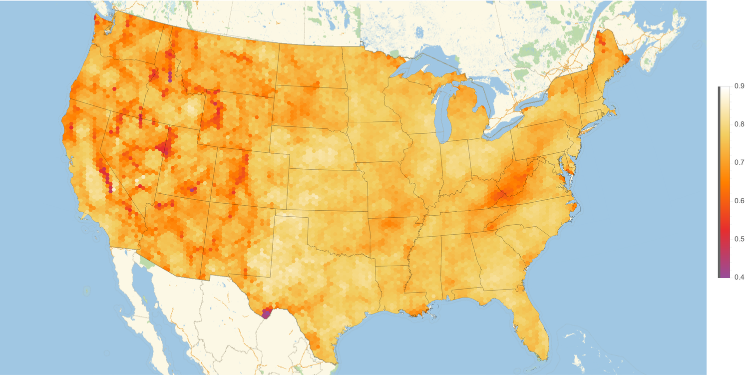
There is a lot to talk about in this map. Route efficiency is significantly lower in mountainous areas like Appalachia, northern Arkansas, and many areas in the West. It is hard to tell whether all of the route inefficiency in the West is attributable to mountains or whether low population density plays a role as well. The Central Valley of California is also particularly visible.

Below is the analogous map of Europe:

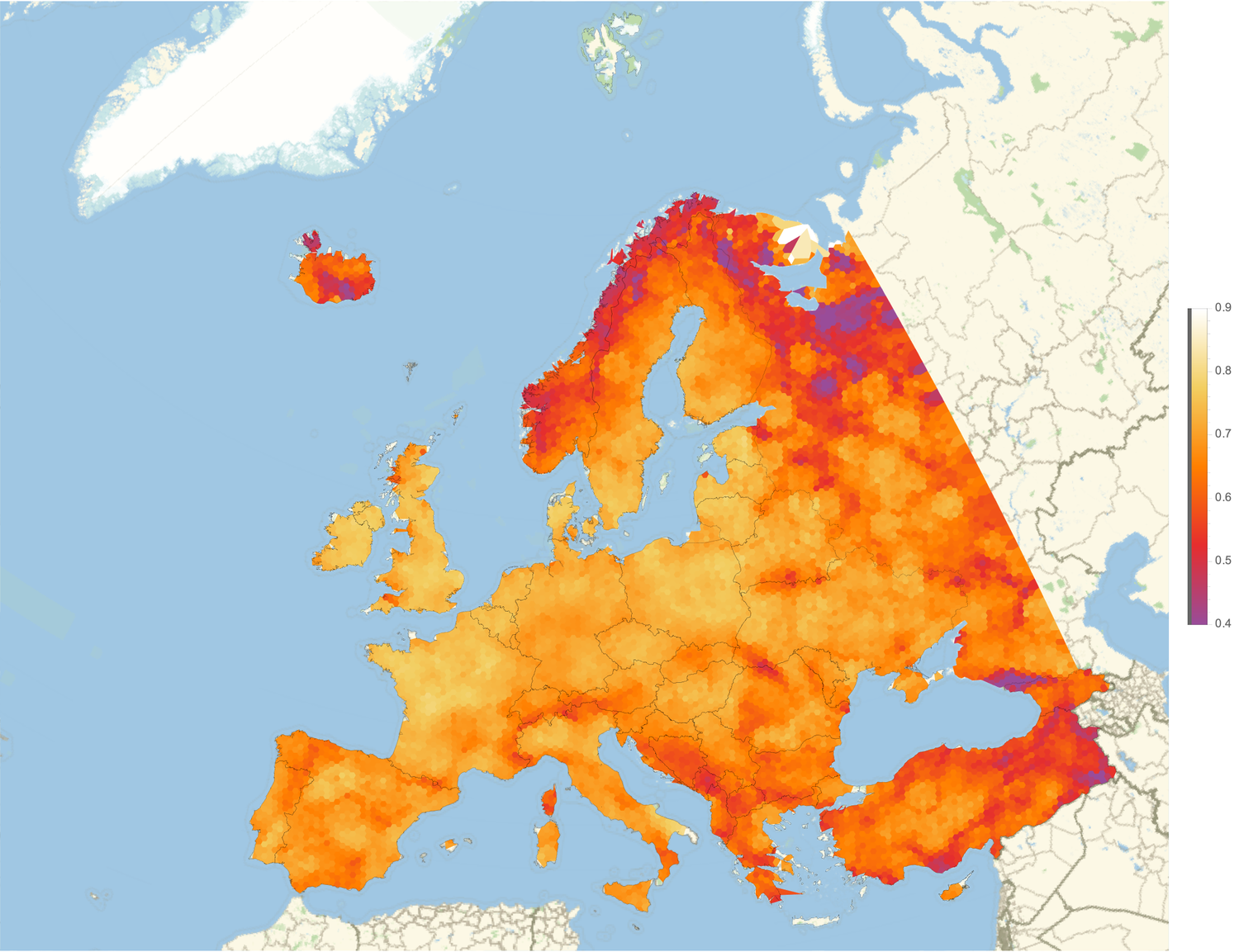
Again, mountains explain much of the variance in route efficiency. The Alps, Carpathian Mountains (between Romania and Ukraine), and Caucasus Mountains (around Georgia) are all clearly visible, as well as mountains in Norway, the Balkans and Turkey. The inefficient routes in western Russia (just east of Finland) seem to be the result of a few large lakes.

Conclusion

To sum up, here are some of the results from this project:

• For routes longer than about 50 miles, route efficiency is approximately uniform, and so geodesic distance is a good approximation for travel distance when dealing with long routes in a country like the US.
• Route efficiency is determined by different factors at different scales. In the short-range regime (<0.2 miles) routes are essentially straight lines and are generally efficient. In the mid-range regime (>0.2 miles but <5 miles) routes rely on a small number of large roads and are generally inefficient. In the long-range regime (>5 miles), routes have a wide variety of major roads to chose from, and are generally efficient.
• Overall route efficiency is lower in Europe compared with the US.
• Route efficiency is negatively affected by mountains.
• Time efficiency can differ significantly from route efficiency.

Code for this project is available as a Mathematica notebook here, and as a PDF here.

(Map data copyrighted OpenStreetMap contributors and available from https://www.openstreetmap.org)